Logistic Regression in ML

Content Highlight:

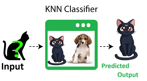
The K-Nearest Neighbors (KNN) algorithm is a powerful, non-parametric, and instance-based supervised learning method used for both classification and regression tasks. It works by finding the K closest data points to a new instance and classifying it based on majority voting. Due to its simplicity, versatility, and interpretability, KNN is widely used in image recognition, recommendation systems, medical diagnosis, and customer behavior prediction.

What is the K-Nearest Neighbors (KNN) Algorithm in Machine Learning?

The K-Nearest Neighbors (KNN) algorithm is a simple yet powerful supervised learning technique used for classification and regression tasks. It operates on the principle of similarity, classifying new data points based on the majority class of their closest neighbors in the feature space.

Unlike traditional models that learn patterns during training, KNN is a non-parametric, instance-based algorithm—meaning it does not make any prior assumptions about the data distribution and does not learn an explicit model. Instead, it stores the entire dataset and makes predictions by computing distances (such as Euclidean distance) between a new data point and its ‘k’ nearest neighbors.

Due to its simplicity, interpretability, and effectiveness, KNN is widely used in various applications like image recognition, recommendation systems, and medical diagnosis. However, it can become computationally expensive for large datasets as it requires calculating distances for every new prediction.

Why Do We Need the K-Nearest Neighbors (KNN) Algorithm?

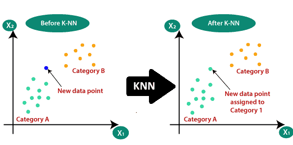
In machine learning, classification problems often involve determining which category a new data point belongs to, based on existing data. Suppose we have two categories, Category A and Category B, and we introduce a new data point x₁. The challenge is to determine whether this new point should be assigned to Category A or Category B.

This is where the KNN algorithm comes into play. KNN helps in classifying a data point based on its nearest neighbors, leveraging similarity measures to make an informed decision. By analyzing the characteristics of nearby points, the algorithm effectively assigns the new data point to the most relevant category.

Classifying a New Data Point Using the K-Nearest Neighbors (KNN) Algorithm

Suppose we have a new data point, and we need to determine the category it belongs to. The KNN algorithm helps in this classification by analyzing the closest neighbors. Consider the diagram below:

Step 1: Choosing the Number of Neighbors (K)

The first step in the KNN algorithm is selecting the number of neighbors (K). In this case, we set K = 5, meaning that we will consider the 5 nearest neighbors to classify the new data point.

Step 2: Calculating the Euclidean Distance

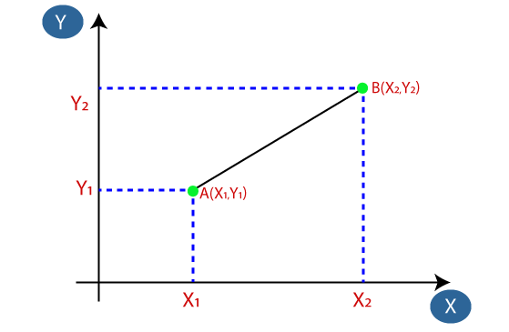
Next, we calculate the distance between the new data point and all existing data points. The most commonly used distance metric in KNN is the Euclidean distance, which measures the straight-line distance between two points in a multi-dimensional space.

The formula for Euclidean distance between two points ( A(X_1, Y_1) ) and ( B(X_2, Y_2) ) is given by:

d(A, B) = √((X₂ - X₁)² + (Y₂ - Y₁)²)

Step 3: Identifying the Nearest Neighbors

After calculating the Euclidean distances, we determine the K nearest neighbors. As shown in the image below, the new data point has:

3 nearest neighbors in Category A
2 nearest neighbors in Category B

Step 4: Assigning the New Data Point to a Category:

Since the majority of the nearest neighbors (3 out of 5) belong to Category A, the new data point is classified as part of Category A.

How to Select the Best Value of K?

Choosing the right value of K is crucial for the performance of the KNN algorithm. Here are some important considerations:

There is no fixed rule for determining the best value of K. It is often selected through experimentation.
A commonly used value is K = 5, which provides a good balance between accuracy and computational efficiency.
A very small value (e.g., K = 1 or K = 2) may be sensitive to outliers and noise, leading to incorrect classifications.
A larger value of K improves stability but may struggle with fine-grained classifications.

By carefully selecting K, we can optimize the KNN model for accuracy and performance, ensuring reliable classifications in various machine learning applications.

How Does the K-Nearest Neighbors (KNN) Algorithm Work?

The KNN algorithm follows a structured process to classify or predict a new data point based on distance-based similarity. The steps involved are:

Step 1: Choose the Value of K:

The first step is selecting the number of nearest neighbors (K) that will influence the classification decision. A smaller K value makes the model sensitive to noise, while a larger K provides smoother decision boundaries.

Step 2: Compute the Distance Between Data Points:

The most commonly used distance metric is the Euclidean distance, which measures the straight-line distance between two points in a multi-dimensional space. Other distance metrics, such as Manhattan distance or Minkowski distance, can also be used depending on the dataset.

Step 3: Identify the K Nearest Neighbors:

Based on the computed distances, select the K closest data points to the new data point.

Step 4: Count the Neighbors in Each Category:

Among the selected K nearest neighbors, count the number of data points belonging to each class.

Step 5: Assign the New Data Point to the Majority Class:

The new data point is classified into the category that has the highest number of neighbors among the selected K.

Step 6: Model is Ready for Predictions

The trained KNN model can now classify or predict future data points based on the majority voting principle.

Key Advantages of KNN:

Simple and Intuitive: Does not require a complex mathematical model to operate.
No Assumption on Data Distribution: KNN is a non-parametric algorithm, meaning it does not assume any underlying distribution of the dataset.
Versatile: Can be used for both classification and regression tasks.
Adaptable: Works well with high-dimensional data when appropriate distance metrics are used.

However, KNN can be computationally expensive for large datasets since it requires calculating distances for each query. Efficient data structures like KD-Trees or Ball Trees can help optimize performance.

KNN remains a fundamental and widely used algorithm for pattern recognition, recommendation systems, and image classification, making it a valuable tool in machine learning.

Since we need a range between -∞ and +∞, we take the logarithm of the equation, resulting in:

log(y / (1 - y)) = b₀ + b₁x₁ + b₂x₂ + ... + bₙxₙ

K-Nearest Neighbors (KNN) Algorithm – Full Detailed Implementation in Python

The K-Nearest Neighbors (KNN) algorithm is a powerful and intuitive supervised learning method used for both classification and regression. This guide explains how to implement KNN from scratch in Python, with detailed code and descriptions.

Step 1: Import Required Libraries:

    
    import numpy as np
    import pandas as pd
    import matplotlib.pyplot as plt
    from collections import Counter
    from sklearn.model_selection import train_test_split
    from sklearn.metrics import accuracy_score

Explanation: We import libraries for data manipulation, visualization, splitting datasets, calculating distances, and evaluating performance.

Step 2: Create a Simple Dataset

    
    data = {
        'X1': [1, 2, 3, 6, 7, 8],
        'X2': [2, 3, 3, 6, 7, 8],
        'Label': ['A', 'A', 'A', 'B', 'B', 'B']
    }
    df = pd.DataFrame(data)
    
    X = df[['X1', 'X2']].values
    y = df['Label'].values

Explanation: This simple dataset includes two features (X1, X2) and class labels. We extract features into X and labels into y.

Step 3: Split the Data

    
        X_train, X_test, y_train, y_test = train_test_split(X, y, test_size=0.33, random_state=42)

Explanation: We split the data into training and testing sets, reserving 33% for testing.

Step 4: Define Euclidean Distance Function

    
    def euclidean_distance(p1, p2):
        return np.sqrt(np.sum((p1 - p2) ** 2))

Explanation: This function calculates the Euclidean distance between two points, which is essential for measuring similarity in KNN.

Step 5: Implement the KNN Logic

    
    def knn_predict(X_train, y_train, X_test, k=3):
        predictions = []
        for test_point in X_test:
            distances = []
            for i, train_point in enumerate(X_train):
                distance = euclidean_distance(test_point, train_point)
                distances.append((distance, y_train[i]))
            distances.sort(key=lambda x: x[0])
            k_nearest_labels = [label for _, label in distances[:k]]
            most_common = Counter(k_nearest_labels).most_common(1)[0][0]
            predictions.append(most_common)
        return predictions

Explanation: For each test point, we:

Calculate distances to all training points
Sort and pick the top K neighbors
Use majority voting to assign the label

Step 6: Make Predictions

    
    y_pred = knn_predict(X_train, y_train, X_test, k=3)
    print("Predictions:", y_pred)

We use our KNN function to predict labels for the test data.

Step 7: Evaluate Accuracy

    
    accuracy = accuracy_score(y_test, y_pred)
    print("Accuracy:", accuracy)

We calculate how many predicted labels match the actual test labels.

Step 8: Visualize the Results

    
    plt.scatter(X_train[:, 0], X_train[:, 1], c=['red' if label == 'A' else 'blue' for label in y_train], label='Training')
    plt.scatter(X_test[:, 0], X_test[:, 1], c=['orange' if label == 'A' else 'green' for label in y_pred], marker='x', label='Predicted')
    plt.xlabel("X1")
    plt.ylabel("X2")
    plt.title("KNN Classification (k=3)")
    plt.legend()
    plt.grid(True)
    plt.show()

This plot visualizes training and test data. Test predictions are marked with an “x”.

Understanding Parameters and Concepts

K (Number of Neighbors): Controls how many nearby points influence classification.
Distance Metric: Typically Euclidean, but can be others like Manhattan.
Lazy Learning: No model is trained; all action happens at prediction time.
Non-Parametric: Doesn’t assume any underlying distribution of data.

Bonus: Use Real Dataset (Iris Example)

    
    from sklearn.datasets import load_iris
    iris = load_iris()
    X = iris.data
    y = iris.target

You can use the same train_test_split and knn_predict() functions with this real-world dataset.

Conclusion:

KNN is a powerful, interpretable, and simple algorithm suitable for many use cases. It requires tuning and may struggle with high-dimensional data, but it's a great starting point for classification tasks. If desired, you can also explore the optimized version using KNeighborsClassifier from Scikit-learn.

←Prev Next→